Loads the dataset used in R. Barro and J.-W. Lee's "Sources of Economic Growth" (1994).

Args:
    return_tuple (bool):  Whether to return the data in a tuple or jointly in a single pandas
                          DataFrame.

Returns:
    pandas.DataFrame or tuple: If `return_tuple` is True, returns a tuple of (X, y), where `X` is a
    DataFrame of independent variables and `y` is a Series of the dependent variable. If False,
    returns a single DataFrame with both independent and dependent variables.
Robert Barro and Jong-Wha Lee’s (1994) dataset has been used over time by other economists, such as by Belloni, Chernozhukov, and Hansen (2011) and Giannone, Lenza, and Primiceri (2021). This function uses the version available in their online annex. In that paper, this dataset corresponds to what the authors call “macro2”.
The original data, along with more information on the variables, can be found in this NBER website. A very helpful codebook is found in this repo.
If you use this data in your work, please cite Barro and Lee (1994). A BibTeX code for convenience is below:
@article{BARRO19941,
title = {Sources of economic growth},
journal = {Carnegie-Rochester Conference Series on Public Policy},
volume = {40},
pages = {1-46},
year = {1994},
issn = {0167-2231},
doi = {10.1016/0167-2231(94)90002-7},
url = {https://www.sciencedirect.com/science/article/pii/0167223194900027},
author = {Robert J. Barro and Jong-Wha Lee},
abstract = {For 116 countries from 1965 to 1985, the lowest quintile had an average growth rate of real per capita GDP of - 1.3pct, whereas the highest quintile had an average of 4.8pct. We isolate five influences that discriminate reasonably well between the slow-and fast-growers: a conditional convergence effect, whereby a country grows faster if it begins with lower real per-capita GDP relative to its initial level of human capital in the forms of educational attainment and health; a positive effect on growth from a high ratio of investment to GDP (although this effect is weaker than that reported in some previous studies); a negative effect from overly large government; a negative effect from government-induced distortions of markets; and a negative effect from political instability. Overall, the fitted growth rates for 85 countries for 1965–1985 had a correlation of 0.8 with the actual values. We also find that female educational attainment has a pronounced negative effect on fertility, whereas female and male attainment are each positively related to life expectancy and negatively related to infant mortality. Male attainment plays a positive role in primary-school enrollment ratios, and male and female attainment relate positively to enrollment at the secondary level.}
}
Load Central Bankers speeches dataset from
Bank for International Settlements (2024). Central bank speeches, all years,
https://www.bis.org/cbspeeches/download.htm.

Args:
    year: Either 'all' to download all available central bank speeches or the year(s)
        to download. Defaults to 'all'.
    cache: If False, cached data will be ignored and the dataset will be downloaded again.
        Defaults to True.
    timeout: The timeout to for downloading each speeches file. Set to `None` to disable
        timeout. Defaults to 120.
    **kwargs. Additional keyword arguments which will be passed to pandas `read_csv` function.

Returns:
    A pandas DataFrame containing the speeches dataset.

Usage:
    >>> load_CB_speeches()

    >>> load_CB_speeches('2020')

    >>> load_CB_speeches([2020, 2021, 2022])
This function downloads the Central bankers speeches dataset (2024) from the BIS website (www.bis.org). More information on the dataset can be found on the BIS website.
If you use this data in your work, please cite the BIS central bank speeches dataset, as follows (Please substitute YYYY for the relevant years):
@misc{biscbspeeches
    author = {{Bank for International Settlements}},
    title = {Central bank speeches, YYYY-YYYY},
    year = {2024},
    url = {https://www.bis.org/cbspeeches/download.htm}
}
# Load speeches for 2020speeches = load_CB_speeches(2020)speeches.head()
Load monetary policy statements from multiple central banks.

Args:
    year: Either 'all' to download all available central bank speeches or the year(s)
        to download. Defaults to 'all'.
    cache: If False, cached data will be ignored and the dataset will be downloaded again.
        Defaults to True.
    timeout: The timeout to for downloading each speeches file. Set to `None` to disable
        timeout. Defaults to 120.
    **kwargs. Additional keyword arguments which will be passed to pandas `read_csv` function.

Returns:
    A pandas DataFrame containing the dataset.

Usage:
    >>> load_monpol_statements()

    >>> load_monpol_statements('2020')

    >>> load_monpol_statements([2020, 2021, 2022])
This function downloads monetary policy statements from 26 emerging market central banks (Armenia, Brazil, Chile, Colombia, Czech Republic, Egypt, Georgia, Hungary, Israel, India, Kazakhstan, Malaysia, Mongolia, Mexico, Nigeria, Pakistan, Peru, Philippines, Poland, Romania, Russia, South Africa, South Korea, Thailand, Türkiye, Ukraine) as well as the Fed and the ECB (press-conference introductory statements). The dataset includes official English versions of statements for 1998-2023 (starting date varies depending on data availability). The original source is Evdokimova et al. (2023). If you use this data in your work, please cite the dataset, as follows:
@article{emcbcom,
    author = {Tatiana Evdokimova and Piroska Nagy Mohácsi and Olga Ponomarenko and Elina Ribakova},
    title = {Central banks and policy communication: How emerging markets have outperformed the Fed and ECB},
    year = {2023},
    institution = {Peterson Institute for International Economics},
    url = {https://www.piie.com/publications/working-papers/central-banks-and-policy-communication-how-emerging-markets-have}
}
# Load monpol statements for 2020speeches = load_monpol_statements(2020)speeches.head()
Loads liquidity risk data from CSV files.

This function loads monthly and weekly liquidity risk data. The data is sourced from the paper
"Using machine learning for detecting liquidity risk in banks" by Rweyemamu Ignatius Barongo and
Jimmy Tibangayuka Mbelwa. The dataset includes data from 38 Tanzanian banks (2010-2021) provided
by the Bank of Tanzania (BOT). Banks are identified by anonymous bank codes.


Parameters:
wide_format (bool): If True, returns data in wide format with pivoted columns. Column names will
    be in the format BANK_CODE__VAR_NAME.

Returns:
dict[str, pd.DataFrame]: A dictionary with keys 'w' for weekly data and 'm' for monthly data.
    The values are pandas DataFrames containing the data for each frequency.
This function loads liquidity risk data from CSV files for 38 Tanzanian commercial banks spanning from 2010 to 2021. The dataset includes both monthly and weekly data provided by the Bank of Tanzania (BOT). The original source is Barongo and Mbelwa (2024).
If you use this data in your work, please cite the dataset, as follows:
@article{BARONGO2024100511,
    author = {Rweyemamu Ignatius Barongo and Jimmy Tibangayuka Mbelwa},
    title = {Using machine learning for detecting liquidity risk in banks},
    journal = {Machine Learning with Applications},
    volume = {15},
    year = {2024},
    doi = {https://doi.org/10.1016/j.mlwa.2023.100511},
    url = {https://www.sciencedirect.com/science/article/pii/S2666827023000646},
}
Load inflation regime data for a given country.

Args:
    country (str|None): The country code (e.g., 'US', 'DE', 'JP').
        If None, loads data for all countries.

Returns:
    A DataFrame containing the inflation regime data for the specified country or all countries.
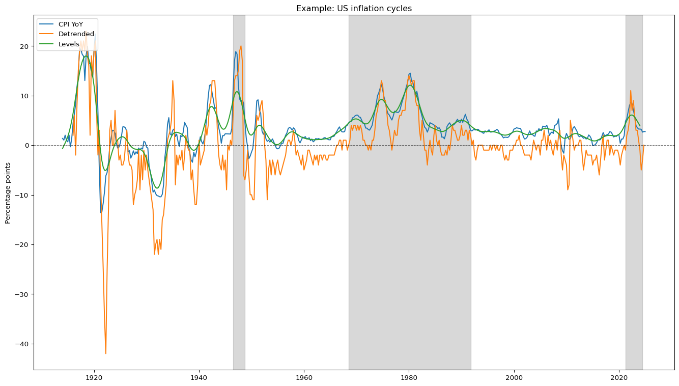
This function provides the data for the Americo et al. (2025) inflation cycle concepts:
cycles in inflation levels, reflecting mostly the low- and medium-frequency components of inflation;
cycles in higher-frequency deviation of inflation from its trend; and
a categorisation of inflation into high and low inflation regimes.
The data also includes the original inflation series used to calculate those cycle measures. These series are also available at the BIS Data Portal.
df_infl = load_inflation_cycles()df_infl.tail()
Date
Country
Series
Value
43913
2025-01-01
TR
Regime
1.000000
43914
2025-01-01
US
CPI YoY
2.736299
43915
2025-01-01
US
Regime
0.000000
43916
2025-01-01
ZA
CPI YoY
2.756116
43917
2025-01-01
ZA
Regime
0.000000
The graph below illustrates the different cycles concepts with US data. The shaded areas are the high inflation periods according to the rule of thumb in Americo et al. (2025).
# Load and prepare datadf_infl_country = load_inflation_cycles("US")pivot_df = df_infl_country.pivot(index='Date', columns='Series', values='Value')if"Detrended"in pivot_df.columns: pivot_df["Detrended"] *=100# Plotfig, ax = plt.subplots(figsize=(14, 8))ax.set_title(f"Example: US inflation cycles")# Plot main seriesfor col in pivot_df.columns:if col notin ['Regime']: ax.plot(pivot_df.index, pivot_df[col], label=col)# Plot zero-line interceptax.axhline(0, color='black', linewidth=0.8, linestyle='--', alpha=0.6)# Regime shading using axvspanif'Regime'in pivot_df.columns: regimes = pivot_df['Regime'] in_regime =False start_date =None# Iterate through the dates and values in the regimes seriesfor date, val inzip(regimes.index, regimes):if val ==1andnot in_regime:# Start of a regime start_date = date in_regime =Trueelif val ==0and in_regime:# End of a regime ax.axvspan(start_date, date, color='gray', alpha=0.3) in_regime =False# If a regime is still active at the end of the data, close itif in_regime: ax.axvspan(start_date, regimes.index[-1], color='gray', alpha=0.3)# Stylingax.legend(loc='upper left')ax.set_ylabel("Percentage points")plt.tight_layout()plt.show()
If you use this data in your work, please cite Americo et al. (2025). A BibTeX code for convenience is below:
@techreport{inflation_cycles,
   author = {Americo, Alberto and Araujo, Douglas KG and Damp, Johannes and Nilsen, Sjur and Rees, Daniel and Schmidt, Rafael and Schmieder, Christian},
   title = {Inflation cycles: evidence from international data},
   series = {BIS Working Paper},
   type = {Working Paper},
   institution = {Bank for International Settlements},
   year = {2025},
   number = {1264}
}
Simulated datasets
Note
All of the functions creating simulated datasets have a parameter random_state that allow for reproducible random numbers.
make_causal_effect (n_samples: 'int' = 100, n_features: 'int' = 100, pretreatment_outcome=<function <lambda> at 0x00000237E211C0E0>, treatment_propensity=<function <lambda> at 0x00000237E211C180>, treatment_assignment=<function <lambda> at 0x00000237E211C220>, treatment=<function <lambda> at 0x00000237E211C2C0>, treatment_effect=<function <lambda> at 0x00000237E211C360>, bias: 'float' = 0, noise: 'float' = 0, random_state=None, return_propensity: 'bool' = False, return_assignment: 'bool' = False, return_treatment_value: 'bool' = False, return_treatment_effect: 'bool' = True, return_pretreatment_y: 'bool' = False, return_as_dict: 'bool' = False)
Generates a simulated dataset to analyze causal effects of a treatment on an outcome variable.

Args:
    n_samples (int): Number of observations in the dataset.
    n_features (int): Number of covariates for each observation.
    pretreatment_outcome (function): Function to generate outcome variable before any treatment.
    treatment_propensity (function or float): Function to generate treatment propensity or a fixed value for each observation.
    treatment_assignment (function): Function to determine treatment assignment based on propensity.
    treatment (function): Function to determine the magnitude of treatment for each treated observation.
    treatment_effect (function): Function to calculate the effect of treatment on the outcome variable.
    bias (float): Constant value added to the outcome variable.
    noise (float): Standard deviation of the noise added to the outcome variable. If 0, no noise is added.
    random_state (int, RandomState instance, or None): Seed or numpy random state instance for reproducibility.
    return_propensity (bool): If True, returns the treatment propensity for each observation.
    return_assignment (bool): If True, returns the treatment assignment status for each observation.
    return_treatment_value (bool): If True, returns the treatment value for each observation.
    return_treatment_effect (bool): If True, returns the treatment effect for each observation.
    return_pretreatment_y (bool): If True, returns the outcome variable of each observation before treatment effect.
    return_as_dict (bool): If True, returns the results as a dictionary; otherwise, returns as a list.

Returns:
    A dictionary or list containing the simulated dataset components specified by the return flags.
make_causal_effect creates a dataset for when the question of interest is related to the causal effects of a treatment. For example, for a simulated dataset, we can check that \(Y_i\) corresponds to the sum of the treatment effects plus the component that does not depend on the treatment:
The pre-treatment outcome \(Y_i|X_i\) (the part of the outcome variable that is not dependent on the treatment) might be defined by the user. This corresponds to the value of the outcome for any untreated observations. The function should always take at least two arguments: X and bias, even if one of them is unused; bias is the constant. The argument is zero by default but can be set by the user to be another value.
And of course, the outcome might also have a random component.
In these cases (and in other parts of this function), when the user wants to use the same random number generator as the other parts of the function, the function must have an argment rng for the NumPy random number generator used in other parts of the function.
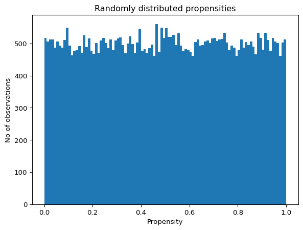
The propensity can also be randomly allocated, together with covariate dependence or not. Note that even if the propensity is completely random and does not depend on covariates, the function must still use the argument X to calculate a random vector with the appropriate size.
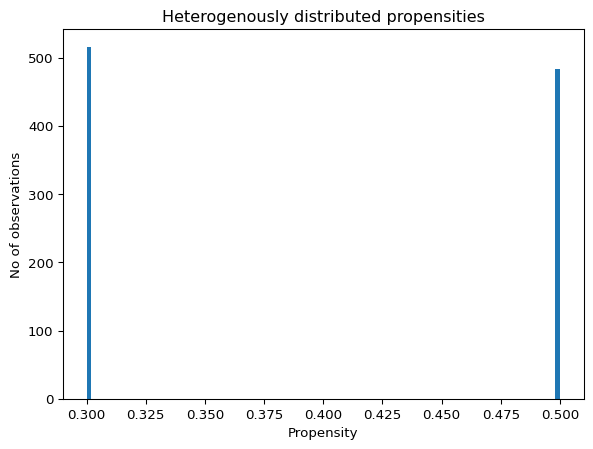
As seen above, every observation has a given treatment propensity - the chance that they are treated. Users can define how this propensity translates into actual treatment with the argument treatment_assignment. This argument takes a function, which must have an argument called propensity.
The default value for this argument is a function returning 1s with probability propensity and 0s otherwise. Any other function should always return either 0s or 1s for the data simulator to work as expected.
While the case above is likely to be the most useful in practice, this argument accepts more complex relationships between an observation’s propensity and the actual treatment assignment.
For example, if treatment is subject to rationing, then one could simulate data with 10 observations where only the samples with the highest (say, 3) propensity scores get treated, as below:
The treatment argument indicates the magnitude of the treatment for each observation assigned for treatment. Its value is always a function that must have an argument called assignment, as in the first example below.
In the simplest case, the treatment is a binary variable indicating whether or not a variable was treated. In other words, the treatment is the same as the assignment, as in the default value.
But users can also simulate data with heterogenous treatment, conditional on assignment. This is done by including a pararemeter X in the function, as shown in the second example below.
Heterogenous treatments may occur in settings where treatment intensity, conditional on assignment, varies across observations. Please note the following:
the heterogenous treatment amount may or may not depend on covariates, but either way, if treatment values are heterogenous, then X needs to be an argument of the function passed to treatment, if nothing else to make sure the shapes match; and
if treatments are heterogenous, then it is important to multiply the treatment value with the assignment argument to ensure that observations that are not assigned to be treated are indeed not treated (the function will return an AssertionError otherwise).
In contrast to the function above, in the chunk below the function make_causal_effect fails because a treatment value is also assigned to observations that were not assigned for treatment.
Argument `treatment` must be a function that returns 0 for observations with `assignment` == 0.
One suggestion is to multiply the desired treatment value with `assignment`.
Treatment effect
The treatment effect can be homogenous, ie, is doesn’t depend on any other characteristic of the individual observations (in other words, does not depend on \(X_i\)), or heterogenous (where the treatment effect on \(Y_i\) does depend on each observation’s \(X_i\)). This can be done by specifying the causal relationship through a lambda function, as below:
Americo, Alberto, Douglas KG Araujo, Johannes Damp, Sjur Nilsen, Daniel Rees, Rafael Schmidt, and Christian Schmieder. 2025. “Inflation Cycles: Evidence from International Data.” Working Paper 1264. BIS Working Paper. Bank for International Settlements.
Barongo, Rweyemamu Ignatius, and Jimmy Tibangayuka Mbelwa. 2024. “Using Machine Learning for Detecting Liquidity Risk in Banks.”Machine Learning with Applications 15. https://doi.org/https://doi.org/10.1016/j.mlwa.2023.100511.
Barro, Robert J., and Jong-Wha Lee. 1994. “Sources of Economic Growth.”Carnegie-Rochester Conference Series on Public Policy 40: 1–46. https://doi.org/10.1016/0167-2231(94)90002-7.
Belloni, Alexandre, Victor Chernozhukov, and Christian Hansen. 2011. “Inference for High-Dimensional Sparse Econometric Models.”arXiv Preprint arXiv:1201.0220.
Giannone, Domenico, Michele Lenza, and Giorgio E Primiceri. 2021. “Economic Predictions with Big Data: The Illusion of Sparsity.”Econometrica 89 (5): 2409–37.